A Comprehensive Guide to Training a Machine Learning Model for Question Answering

by Batya Stein & Nicholas Greenspan

Batya Stein is a rising junior at Princeton University studying Computer Science and English Literature. Her research interests include Natural Language Processing and Software Engineering and Design. Previously, she has interned at a non-profit, designing a project to interface between its CRM softwares. When not coding, she enjoys drawing, swimming, and reading fiction. Batya was one of NLMatics’ 2020 summer interns.


Nicholas Greenspan lives in New York City and is a freshman at Rice University who is majoring in computer science. Nicholas is interested in Machine Learning, Natural Language Processing, and their applications to various fields. Nicholas recently worked at the UTHealth School of Biomedical Informatics working on a Natural Language Processing project to help doctors find relevant treatments for their patients, and is excited to work on more interesting and meaningful problems at NLMatics. Outside of CS, Nicholas likes to read, play ice hockey, and listen to many genres of music including indie rock and electronic. Nicholas was one of NLMatics’ 2020 summer interns.

---

A Comprehensive Guide to Training a Machine Learning Model for Question Answering:

Fine-tuning ALBERT on Google Natural Questions

Contents:

1. Setting up the EC2 Instance
   • Choosing and launching EC2 Instance
   • Preparing instance for training
   • Setting up Wandb logging
2. Downloading and Formatting Data
   • About the datasets
   • Downloading the data
   • Processing from zip file
   • Reformatting Google Natural Questions to SQuAD format
3. Training the Model
   • Model comparisons
   • Understanding run_squad.py parameters
   • Common errors encountered during training
   • Restoring from a checkpoint
   • Understanding model outputs
   • Downloading your model and uploading to an S3 bucket

Intro:

Feel like a machine learning question answering system could give your business a boost? Just interested in trying out revolutionary AI tech? You’ve come to the right place. Training your first deep learning model can feel like navigating a labyrinth with no clear start or finish, so we’ve made a highly detailed guide to save you time, energy, and a lot of stackoverflow searches. This is a comprehensive guide to training a ML question answering model that will walk you through every step of the process from cloud computing to model training. We will use AWS for our cloud computing necessities, and Huggingface’s transformers repository to access our ALBERT model and run_squad.py script for training.

Why do I care? What AI can do for you:

Extracting information from long text documents can be a time consuming, monotonous endeavour. A revolutionary cutting edge technology, NLP Question Answering systems can automate this process, freeing you up to use that information to make decisions to further your business. Given a piece of text and a question, a Question Answering system can tell you where the answer lies in the text, and even tell you if the answer isn’t present at all! If this technology interests you, and you want to apply it at a business-level scale, you should definitely check out NLMatics’ product at https://www.nlmatics.com/.

We ran the model training described here during our summer engineering internship at NLMatics. Currently, one of the most popular Question Answering transformer models is trained on the SQuAD dataset, and we were curious to see if training on Google Natural Questions could give us more effective results. (As of this post, there are no ALBERT models pretrained on Google Natural Questions available for use online.) Along the way, we learned a lot about the ins and outs of model training, memory management, and data-logging.

Huggingface’s transformers github repository, an open source resource for training language models, greatly simplifies the training process and puts many essential materials all in one place. Huggingface provides scripts for training models on different datasets, which saves you the labor of writing your own. In order to train on a new dataset while still making use of Huggingface’s run_squad.py script and functions for evaluating SQuAD training metrics, we converted the Google Natural Questions dataset into the same format as SQuAD. For this reason, this guide can help you whether you want to use Google Natural Questions, SQuAD, or any other question answering dataset to train a transformer model.

To learn more about machine learning or language models, see the links below.
Machine Learning
Transformer architecture (BERT)

To learn more about the datasets we worked with, see the links above or our blog post comparing the characteristics of both sets.

PART 1: SETTING UP THE EC2 INSTANCE

Choosing And Launching An EC2 Instance:

To start our model training, we have to choose the right platform (one with a bit more computing power than a personal computer)

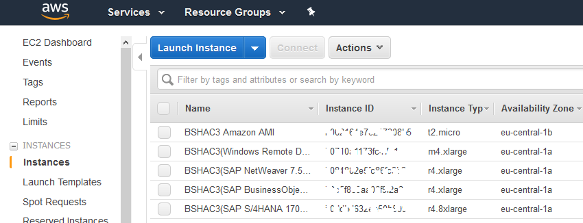List of instances in EC2 dashboard

What is AWS EC2?

Amazon Web Services’ EC2 service allows users to utilize cloud computing power from their local machines. An On-Demand EC2 Instance provides a virtual server that charges per hour that instance is running.

Instance types and costs

To choose an instance for your use case, consider its GPU and vCPU capacities, storage space, and cost. For our training, we considered P and G- type instances, since both classes come with GPU power. P2/P3 instances have up to 16 GPUs (P3 is the latest generation and comes at a slightly higher cost). G4 instances have up to 4 GPUs, but are more cost effective for larger amounts of memory. Note that if you’re using CUDA, a platform for computing with GPU power often used in machine learning applications, the maximum number of GPUs it will run on is 8, due to limitations in the “peer-to-peer” system. We chose the p2.8xl instance, which has 8 NVIDIA K80 GPUs and 96GB of storage.

Instance	GPUs	GPU Type and total GPU memory	vCPUs	RAM	Linux Pricing (USD/HR)
p2.xlarge	1	NVIDIA K80 GPU (12GiB)	4	61 GiB	0.9
p2.8xlarge	8	NVIDIA K80 GPU(96GiB)	32	488 GiB	7.2
p2.16xlarge	16	NVIDIA K80 GPU (192GiB)	64	732 GiB	14.4
p3.2xlarge	1	NVIDIA Tesla V100 GPU (16GiB)	8	61	3.06
p3.8xlarge	4	NVIDIA Tesla V100 GPU (64GiB)	32	244	12.24
p3.16xlarge	8	NVIDIA Tesla V100 GPU (128GiB)	64	488	24.48
g4dn.xlarge	1	NVIDIA T4 Tensor Core GPU (16GiB)	4	16	0.526
g4dn.8xlarge	1	NVIDIA T4 Tensor Core GPU (16GiB)	32	128	2.176
g4dn.12xlarge	4	NVIDIA T4 Tensor Core GPU (64GiB)	48	192	3.912
g4dn.16xlarge	1	NVIDIA T4 Tensor Core GPU (16GiB)	64	256	4.352

Account limits

Before launching an instance, be aware that each type has a specific vCPU capacity that it needs to run, which can be found in the chart above. However, all AWS accounts have automatic limitations on the number of vCPUs that can be allocated per instance class. Current account limits can be viewed in the EC2 section of the “Service Quotas” tab in the AWS console. Make sure you are in the same region you plan on starting your instance in, then check the “applied quota value” for “Running On-Demand P instances” (or instance class of your choice). If the current vCPU limit isn’t large enough to launch your instance, use the “Request Limit Increase” button to request the necessary number of vCPUs. In our experience, requests can take up to 48 hours to be filled, so request increases in advance of when you plan to start your training.

Once the limit is increased, you can launch your instance from the AWS EC2 console. Choose a platform with deep learning capabilities - we needed CUDA and a PyTorch environment, so we chose the Deep Learning AMI (Amazon Linux) Version 30.0. Next, choose instance type, and add additional storage if desired. Then configure the security group to allow from incoming connections from your IP address to the instance, by adding a rule of Type “SSH” with Source “My IP Address”, which automatically fills in your IP for you. You can also add additional rules to the security group later if needed to give others access to the instance. Do so by choosing your instance from the console instance list. Under its description, click its security group, then from the pulldown menu in the security groups list choose actions -> edit inbound rules -> add SSH rule, with IP of the person who needs access as the source.

Key-pair security file

To secure connections to your instance, create a key-pair file. In order to work, the key must not have public security permissions, so once you’ve downloaded the file, go to your terminal, navigate to the directory that the file is stored in, and run chmod 400 keypair-file-name.

You can then connect to the instance from your terminal/ command-line by selecting the instance in the console list and running the example command given by the connect button, which will look like ssh -i”xxx.pem” EC2-user@EC2-xx-xx-xxx-xxx.us-region.compute.amazonaws.com. (When logging onto the server for the first time, you may get a warning that “The authenticity of host… can’t be established” but this should not be a security issue since you are instantiating the connection directly from AWS.)

IAM roles (sharing AWS resource access)

If you want to give someone else access to the instance without giving them your account login information, you can create an IAM role in the IAM console. In the Users menu, add a User with AWS Management Console access, give user all EC2 permissions and then share the role’s login information. Once you start using your instance, you can monitor the costs or credits used, with the AWS cost explorer service. Make sure to stop the instance when not in use to avoid extra charges!

Preparing The Instance For Training

Before we can get started with training, we’ll need to load all the necessary libraries and data onto our instance.

Upload training data

Prepare for training by connecting to your EC2 instance from the terminal of your choice and creating a directory inside it to store the data files in. (See section II, on downloading and reformatting data, to learn how to get your data into the right format before you start working with it.) Upload your training and dev sets into the directory (in json format). Upload the training script, which can be found in the Transformers github repo, onto the instance. Lastly, create a new directory that will be used to store the evaluations and model checkpoints from the script’s output.

Note that if you’ve previously trained a model of the same type on your EC2 instance, there will be a cached datafile with a name like “cached_dev_albert-xlarge-v2_384”. If you’re training on a different dataset than you used in the previous training, make sure to delete the cached file, otherwise the script will automatically load the data from it and you’ll end up training on different data then you meant to.

File transferring

To upload and transfer files between an EC2 instance and local computer you can use the following terminal commands. (Run these commands while the instance is running, but in a separate terminal window from where the instance is logged in.)

From local -> EC2 – run the command scp -i /directory/to/abc.pem /your/local/file/to/copy user@EC2-xx-xx-xxx-xxx.compute-1.amazonaws.com:path/to/file

From EC2 -> local (for downloading your model checkpoints, etc.) run scp -i /directory/to/abc.pem user@EC2-xx-xx-xxx-xxx.compute-1.amazonaws.com:path/to/file /your/local/directory/files/to/download

Another option is to use FileZilla software for transferring files. This post explains how to set up a connection to the EC2 instance through Filezilla with your pem key.

Library installations

Prepare your environment by downloading the libraries needed for the run_squad script. Run the following commands in the terminal of your choice, while logged into your instance:

source activate env-name

• This command activates a virtual environment. Choose one of the environments that come pre-loaded onto the instance, listed when you first log into the instance from your terminal. Since run_squad.py relies on PyTorch, we used the environment “pytorch_latest_p36”. PyTorch is a python machine learning library that can carry out accelerated tensor computations using GPU power.

pip install transformers

• Transformers is the Huggingface library that provides transformer model architectures that can be used with PyTorch or tensorflow. The transformers library also has processors for training on SQuAD data, which are used in the run_squad.py script.

pip install wandb

• Wandb is web app that allows for easy visualization of training progress and evaluation graphs, lets you see logging output from terminal, keeps track of different runs within you project, and allows you to share results with others (We’ll talk more about how to use Wandb to view your results in the next section!)

pip install tensorboardX

• The run_squad.py script uses the tensorboard library to graph evaluations that are run as training progresses. We’ll sync wandb with tensorboard so the graphs can be seen directly from the wandb dashboard.

git clone https://github.com/NVIDIA/apex cd apex pip install -v --no-cache-dir ./

• Apex is a pytorch extension that allows scripts to run with mixed-floating point precision (using 16 bit floats instead of 32 bit in order to decrease RAM usage)

Setting Up Wandb Logging

You’re going to want to keep track of your training as it happens - here’s where we’ll set that up.

Wandb (Weights & Biases) provides a web-based platform for visualizing training loss and evaluation metrics as your training runs. Checking up on metrics periodically throughout training lets you visualize your progress, and course-correct if your loss suddenly swings upwards, or your metrics take a dramatic turn down.

First you’ll want to create a free account on wandb’s website. Then, to connect your wandb account to your EC2 instance, go to the wandb website settings section and copy your api key. Log into your EC2 instance from your terminal and run the command wandb login your-api-key.

Next, we’ll edit the run_squad.py script to integrate wandb logging. (You can edit it on your computer before uploading to the instance in the terminal editor of your choice after uploading it.)

• Add import wandb to the library imports.
• Before line 742 (sending model to cuda), add wandb.init(project="full_data_gnq_run", sync_tensorboard=True)). This will create a wandb project with the given name. Each time the script is rerun with the same project name will show up as a new run in the same project. Setting sync with tensorboard to true automatically logs the tensorboard graphs created during training to your project page.
• In the next line, add wandb.config.update(args) to store all the arguments and model parameters inputted to the script
• On line 759, after sending model to device, add wandb.watch(model, log='all'), which saves the weights of the model to wandb as it trains.

Now that you’ve added wandb statements into your script, you can watch your training progress from the wandb project dashboard. Two particularly helpful sections are the charts, where you can see loss and evaluation metrics, and the logs, where you can see the output of your script as it runs to track what percent complete your training is.

Wandb charts from our Google Natural Questions training

PART 2: DOWNLOADING AND FORMATTING DATA

We’re going to download the data for the model to train on, and tweak it a bit to get it into the right format.

(Note that a lot of the information in this section is about Google Natural Questions, but the same tips for handling and reformatting large datasets could apply to any dataset of your choice.)

About the Datasets

Both SQuAD and Google Natural Questions are datasets containing pairs of questions and answers based on Wikipedia articles. Fundamentally, they serve the same purpose - to teach a model reading comprehension by having it locate answers within a large amount of text.

However, there are also some interesting differences between the two datasets that made us want to experiment with training a model on Google Natural Questions instead of SQuAD. To start, Google Natural questions has about twice the amount of training data as SQuAD does. SQuAD gives paragraphs from Wikipedia articles as context for its answers and has multiple questions per article, while Google Natural Questions gives entire Wikipedia articles for context, and only has one question per article. Additionally, all of SQuAD’s answers are short (about a sentence long), but Google Natural Questions has some questions with short answers, some with long answers, some with yes-no answers, and some with combinations of all of the above.

Example of a SQuAD 2.0 datapoint:

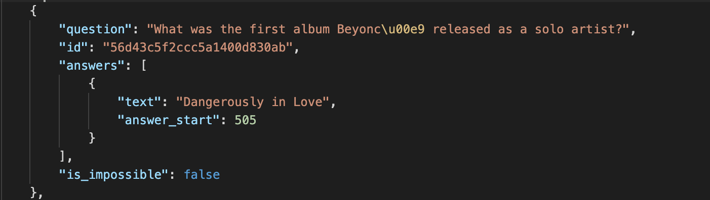
Answer_start indicates the character count where the answer is located in the context. Some questions in SQuAD 2.0 are flagged is_impossible, if answers to them cannot be found in the given context.

To learn more about the differences between the datasets, their compositions and the decisions we made when reformatting, please see Nick’s SQuAD vs. Google Natural Questions blog post.

Downloading the Data

Or, how to actually access 40GB worth of question-answer pairs for training

Our goal was to train on the Google Natural Questions dataset using Huggingface’s run_squad.py script. To do so, we first had to convert the Google Natural Questions examples into SQuAD format. (This might seem like a convoluted approach but it’s actually one of the easiest ways to train with a new question answer dataset, since the Huggingface transformers library has functions specifically designed to process and evaluate SQuAD-formatted examples.)

To get the data for reformatting, you can either download it directly to your computer or you can upload it to an Amazon S3 bucket and stream it into your reformatting script from there. S3 buckets are an AWS service that allow you to store data in the cloud and share it with others.

Downloading Google Natural Questions to your local computer

If you have 40 gb of room on your local computer, you can download all the GNQ files using the google command line interface gsutil as described on the GNQ homepage. (We didn’t want to use the simplified train data that is directly linked to on the homepage because it didn’t give all the information we needed for our reformatting script.

Alternatively, you can download the files directly within your reformatting script, as demonstrated in our code, by using the python request library to download the files from the urls of the google bucket where they are publicly stored.

Streaming Google Natural Questions from an S3 Bucket

If you don’t have enough storage to download the files to your local computer, you can use gsutil to upload the data to an Amazon S3 bucket and then stream the data into your python reformatting code from the bucket without needing to download it first. To do so, follow these steps:

• Make an AWS S3 bucket to hold the data
• Install gustil and AWS CLI, which are command line interaces for Google and AWS, respectively
• Configure your AWS cli following these instructions
• Check that everything works by running aws s3 ls in your terminal, which displays the list of buckets associated with your AWS account
• Run gsutil -m cp -R gs://natural_questions/v1.0 s3://your_bucket_name to download all data, or to download individual files replace gs://natural_questions/v1.0 with gs://natural_questions/v1.0/dev/nq-dev-00.jsonl.gz (there are 5 dev files altogether, so repeat this command through “dev-04”) and gs://natural_questions/v1.0/train/nq-train-01.jsonl.gz (there are 50 train files altogether, so repeat the command through “train-49”)
• To stream the data from the s3 bucket in a python script, follow this tutorial

Downloading SQuAD Data

If you want to use the SQuAD dataset instead of Google Natural Questions to follow our tutorial, the data can be downloaded from https://rajpurkar.github.io/SQuAD-explorer/ using the links “Training Set v2.0 (40MB)” and “Dev Set v2.0 (4MB)” for the training and dev sets respectively on the left hand side bar.

Processing Data from a Zip File

The Google Natural Questions training files take up 40 GB even when contained in gzip (similar to zip) format. When unzipped into json format, any one of the files is large enough to likely crash whatever program you try to open them with. Therefore, when processing Natural Questions or any similarly large dataset in python, it is easiest to do so straight from a zip file.

To process a gzip in python, import gzip library and use a command such as

with gzip.open('v1.0_train_nq-train-00.jsonl.gz', 'rb') as f:
	for line in f: 
	    ...

To process a zip file, import zipfile library and use a command like

with zipfile.ZipFile(“filename.zip”,”r”) as z:
    with z.open(“unzippedfilename”) as f:
   	    for line in f:
   	        ...

Reformatting Google NQ Data to SQuAD Format

We wrote a python script that can be found here for reformatting the data on our local computers before uploading the data to our EC2 instance. Since the way boths datasets are formatted is so different, we had to make certain decisions about how to reformat Google Natural Questions, like using the long answers as context and the short answers as answers. (Entire Wikipedia articles took way too long to process.)

To hear more about the decisions we made when reformatting, see our code, linked above, and the SQuAD vs. Google Natural Questions blogpost.

PART 3: TRAINING THE MODEL

Model Comparisons

There are a number of different deep learning language models out there, many of which are based on BERT. For our purposes we choose ALBERT, which is a smaller and more computationally manageable version of BERT. For more detailed information on the different language models see here: (https://github.com/huggingface/transformers#model-architectures).

Understanding the Parameters of run_squad.py

Almost time to launch the training!

Script parameters

Below is a list of parameters that we used for running run_squad.py. Note that not all of the parameters are necessary (only model_type, model_name_or_path and output_dir are needed for the script to run).

--model_type: This is the type of model you are using. The main types are (‘distilbert’, ‘albert’, ‘bart’, ‘longformer’, ‘xlm-roberta’, ‘roberta’, ‘bert’, ‘xlnet’, ‘flaubert’, ‘mobilebert’, ‘xlm’, ‘electra’, ‘reformer’). We used ‘albertxlv2’.

--model_name_or_path: This is where you indicate the specific pretrained model you want to use from https://huggingface.co/models, we used albert-xlarge-v2. A list of Huggingface provided pretrained models is here https://huggingface.co/transformers/pretrained_models.html. If you want to load a model from a checkpoint, which we will explain how to do later, you would provide the path to the checkpoint here.

--output dir: This is where you specify the path to the directory you want the model outputs to go. The directory should be empty.

--do_train: This indicates that you want to train your model.

--do_eval: This indicates that you want to evaluate the performance of your model.

--train_file: This is the path to the file with your training data.

--predict_file: This is the path to the file with your evaluation data.

--learning_rate: Determines the step size when moving towards minimizing the loss. We used 3e-5.

--num_train_epochs: Determines the number of times you want to go through the dataset. For our training the metrics started to plateau around the end of the third epoch. We would recommend 3 to 5 epochs, but you can stop training prematurely if you see your metrics plateauing before the training has finished.

--max_seq_length: The maximum length of a sequence after tokenization. We used 384, which is the default.

--threads: The number of vCPU threads you want to use for the process of converting examples to features. Check how many vCPU threads you have, it should be the number of vCPU cores times 2. We used 128 threads.

--per_gpu_train_batch_size: The batch size for training you use per gpu, aka the number of examples the model will look at in one iteration. That is if you have 4 gpus and your --per_gpu_train_batch_size is 4, your total batch size will be 16. A larger batch size will result in a more accurate gradient, but a smaller batch size will make the training go faster and use less memory. We used 1.

--per_gpu_eval_batch_size: Same thing as per_gpu_train_batch_size except for evaluation. We used 8.

--version_2_with_negative: If you are using the SQuAD V2 dataset with negative examples use this flag.

--evaluate_during_training: Determines if you want to evaluate during training, but note that this will only work if you are only using 1 gpu due to averaging concerns.

--fp_16: Determines if you want to use 16 point precision instead of the default 32 point precision. This will decrease the amount of ram you use and decrease the training time. Note if you want to use this flag you must have Nvidia apex installed from https://www.github.com/nvidia/apex (as described above).

--gradient_accumulation_steps: Makes gradient descent more stable (in a similar training to the one described here, we used 4)

Screen command

We know you’re probably excited to start training, but here are a few helpful commands before jumping in.

Before you start training your model there is one important terminal functionality you should use. Since you don’t want the training process to stop every time your terminal disconnects from the EC2 instance, which will happen after periods of inactivity, you need to disconnect the process of training the model from the EC2 terminal. To do this, go to the terminal logged into your EC2 instance and run the command screen which will create a blank terminal screen. Once you have done that you can run the command to start the training.

(Note that in order for a virtual environment to work within the screen, you must be running the base environment outside of the screen. Before activating the screen, if you are in a virtual environment, run the command conda activate to return to the base environment, and only activate your virtual environment once you have entered the screen).

The command consists of python run_squad.py followed by all of the flags you want to use for your training.

Here is the command we ran:

python run_squad.py --model_type ALBERTxlv2 --model_name_or_path ALBERT-xlarge-v2 --do_train --do_eval --evaluate_during_training --train_file ~/real_data/modified_GNQ_las_as_context_1_10th_train.json --predict_file ~/real_data/modified_GNQ_las_as_context_1_10th_dev.json --learning_rate 3e-5 --num_train_epochs 7 --max_seq_length 384 --doc_stride 128 --output_dir ~/reformatted_outputs --per_gpu_eval_batch_size=8 --per_gpu_train_batch_size=1 --fp16 --threads 128 --version_2_with_negative

Once you start the training and see that it has started without any initial errors you can hit control a and then control d which will return you to your previous terminal screen with the training running in the background. You can now disconnect from the EC2 instance without affecting the training. Please note that you must not actually turn the instance off during training or the training will be halted. To reconnect to the screen where the training is running, run the command screen -r. It is a good idea to check in on the training once in a while to make sure it has not halted, which can be easily accomplished by looking at the wandb logging, and you can even set your wandb account to send you email alerts if the training fails.

Common Errors We Encountered and How to Fix Them

To save you much of the frustration we endured, here are some errors we encountered and information on how to deal with them.

If you want to be proactive about your training you could look through this section before you start the training and take measures to prevent any possible errors you may feel are likely to come up.

The two main errors we encountered were running out of memory (RAM) and computer storage within our EC2 instance. (The commands presented here are meant to be run while logged into your instance, and assume that your instance runs on a linux operating system.)

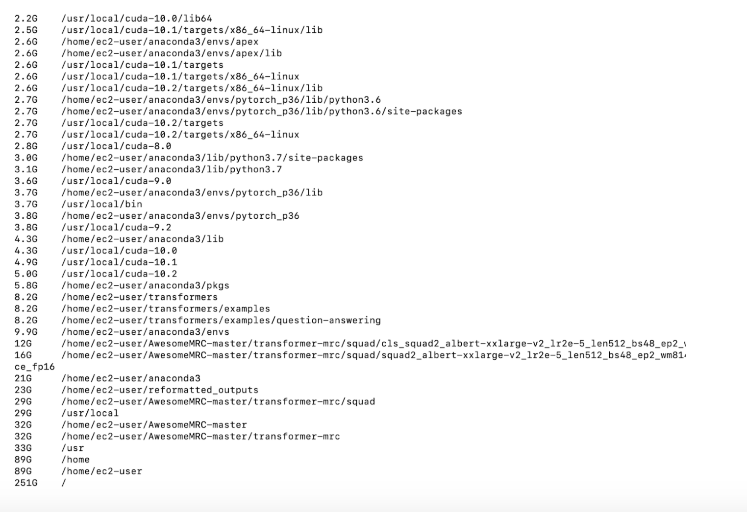
How to manage storage:

To see your current storage usage, run the command df -h. To find the largest files on your instance, run sudo du -x -h / | sort -h | tail -40

If you find yourself running out of storage there are a number of ways to get around it.

Firstly, you could simply delete unneeded files on your amazon aws instance. To do that, navigate to the directory the files or folder you want to delete are located. Then run the command rm 'filename' to delete a single file, or the rm -R ‘foldername’ if you want to delete a folder and all files in it. You can also delete virtual environments you aren’t using that come preinstalled on the EC2 instance. (For running run_squad.py, you only need the pytorch_latest_p36.) Do so by running the command ‘conda remove –name ‘myenv’ –all’ where myenv is the name of the environment you’d like to delete. A list of all installed environments is shown when starting up the instance.

Another method is to simply add more storage to your machine through AWS. You can do this by simply going to the “volumes” section under the elastic block store header in the EC2 section of AWS. Once you are there select the instance you want to add more storage to, click the actions drop down menu, and then select modify volume. From here you can add as much storage as you like, but keep in mind you will be charged for it. See pricing info here: https://aws.amazon.com/ebs/pricing/. Note that you can only increase the volume size and not decrease it, so once you add more storage there is no going back.

There are other methods for dealing with lack of storage issues, such as saving checkpoints to an s3 bucket as training runs, but we did not end up needing to use them.

How to manage memory (RAM, different than storage space):

To figure out your free memory in your instance at a given moment run the command free -h. A good way to keep track of your memory usage throughout the run is to look at the wandb logging in the system section. If you keep encountering out of memory issues, there are a few ways to get around it.

A way of increasing your overall memory is to use something called swap space. If you are not familiar with swap space, it basically involves partitioning part of your storage to be used for memory. A detailed guide can be found here: https://www.digitalocean.com/community/tutorials/how-to-add-swap-space-on-ubuntu-16-04.

One method to decrease memory usage is to decrease your batch size. Note that if you are having out of memory issues in the convert examples to features part of the training process this will not help.

Another method to decrease memory usage is to run the run_sqad.py script with the –fp_16 flag on if you are not already.

If you are getting out of memory issues in the convert examples to features part of the training process, it might be necessary to decrease the size of your dataset.

One final word of advice to avoid random errors is to make sure that you have the most recent version of the transformers library installed, and you are using the most recent run_squad.py script. We encountered some errors related to mismatched versions.

Note: Besides looking at the Wandb logging, you can use the command nvidia-smi to view available gpus and current gpu usage on your instance, and the command top to see your current cpu usage, as well as your memory usage.

Restoring Training From a Checkpoint

Annoyed you have to start from the beginning after your model training failed? Well, you don’t have to! Here’s how you can resume training from a checkpoint.

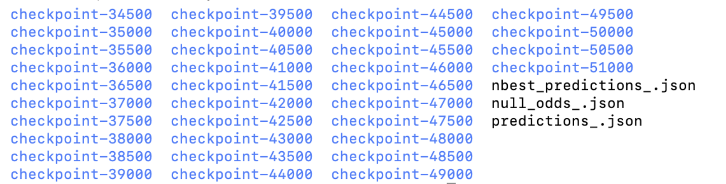
After every 500 examples that the model trains on, it will output a “model checkpoint” that is a representation of the model at that point in training. The model checkpoints can be found in the output folder, and each one is stored in a folder called “checkpoint-x” where x is the number of examples the model had looked at when that checkpoint was generated. Resuming training from a checkpoint can save you a lot of time and convenience.

If you encounter an error and want to pick up the training where you left off, or just want to resume training from a checkpoint for any other reason, here’s how to do it.

All that is necessary is to run the same command you ran to start the training except --model_name_or_path must be set to the path to the folder for the checkpoint you want to resume training from. For example if your output folder is called outputs-2 and you want to resume training from checkpoint-1500 you should have --model_name_or_path /path_to_outputs_folder/outputs-2/checkpoint-1500. For consistency, if you’re restarting training from the middle, you may want to see what the learning rate was at the checkpoint you’re using (on wandb), and use that as the starting learning rate for your new training.

Note that if you do end up stopping your training early due to the metrics leveling off, you will have stopped the script before it reached the evaluation section, so if you want the evaluation results you will have to run the script again with only the –do_eval flag, and not the –do_train flag, and –model_name_or_path should be set to the path to the checkpoint you want to evaluate.

Also note that if you previously ran an evaluation on a checkpoint, and now you want to evaluate that checkpoint using a different data file than you originally used, be sure to delete the any cached dataset files associated with that checkpoint (which will have names like “cached_dev_checkpoint-7000-v2_384”), so that your evaluation runs on the new data file instead of the old cached data.

Understanding Your Model Outputs

What’s the point in training a model if we can’t understand what it’s telling us? Here is a primer on comprehending model terms.

Understanding some run_squad evaluation metrics

These metrics allow you to judge how well your model learned the dataset that you gave to it:

• ‘Exact’ - compares answers that the model predicts for the dev set questions with the real answers, returns percentage of answers that model predicted correctly (eg answer spans match exactly) out of total dev set examples
• ‘F1’ - f1 is an accuracy measure that equals 2((precisionrecall)/(precision+recall)), where precision is the number of true positives over all positive results that the test returns, and recall is the number of true true positives over everything that should have been identified as positive. Here, precision and recall are computed by splitting the correct answers and the predicted answers into tokens by word. The number of tokens that appear in both answers is counted. This intersecting token count is divided by the number of tokens in the predicted answer to find the precision, and divided by number of tokens in the real answer to find recall. The final f1 score returned is the sum of f1 scores for each example in the dev set divided by the total number of examples.
• ‘Total’ - total number of examples in dev set
• ‘HasAns_exact’ - average exact score (computed as above) but only taking the average for all examples in the dev set that have answers (e.g. not impossible)
• ‘HasAns_f1’ - average f1 score over all examples in dev set that have answers
• ‘HasAns_total’ - total # of examples in dev set that have answers
• ‘NoAns_exact’ - average exact score over all examples in dev set that have no answer (e.g. are impossible) ‘NoAns_f1’ - average f1 score over all examples in dev set that have no answer
• ‘NoAns_total’ - total number of examples in dev set that have no answer

Understanding the final model outputs

Every checkpoint folder has files containing information about the model, optimizer, tokenizer, scheduler, tokens, and the training arguments. When the model has finished evaluating, it will output a predictions_.json file, a nbest_predections_.json file, and a null_odds_.json if you are using the SQuAD V2 dataset. The predictions file contains the model prediction for each example in the evaluation file, while the nbest_predictions file contains the n best predictions for each example in the evaluation file, where n is by default 20.

Downloading Your Model/ Uploading to S3 Bucket

Congratulations! You’ve officially trained a ML model for Question Answering! Now that we have our model, where should we store it for future use?

Once your model is trained, the last step is to download it from the EC2 instance so that you and others can access it. (Once an EC2 instance is deleted the information on it also is, so be sure to save the model information you want before terminating your instance for good.) You can save all checkpoints that were stored throughout training, or you can choose to save only the best checkpoint based on evaluation metrics (be aware that the best checkpoint is not necessarily the last.)

To download the checkpoints to your local computer, use the scp command described above for file transfers from SSH. In order to share the model with others, or to upload it to Huggingface for public use, you will need to upload it to an Amazon s3 bucket. You can upload locally downloaded files to the s3 bucket using the s3 section of the AWS console.

Alternatively, you can download the AWS client software onto your EC2 instance and upload the model files directly to a bucket without first downloading to your local computer. Do this by creating an s3 bucket from the s3 web console. Then connect the s3 bucket to your instance using an IAM role and the AWS cli software by following the steps outlined in this post. Once you have downloaded AWS cli, you can use the command “aws s3 cp filetocopy.txt s3://mybucketpath” to copy files into the bucket. Set permissions for public access using the command flags described here, or set permissions directly from the s3 web console.

Sources

https://medium.com/@dearsikandarkhan/files-copying-between-aws-EC2-and-local-d07ed205eefa – file transfer between EC2 and local
https://www.digitalocean.com/community/tutorials/how-to-add-swap-space-on-ubuntu-16-04 – adding swap space
https://medium.com/@arnab.k/how-to-keep-processes-running-after-ending-ssh-session-c836010b26a3 – screen command
https://docs.aws.amazon.com/AWSEC2/latest/UserGuide/authorizing-access-to-an-instance.html – authorizing inbound traffic to instance
https://github.com/huggingface/transformers#run_squadpy-fine-tuning-on-squad-for-question-answering https://machinelearningmastery.com/classification-accuracy-is-not-enough-more-performance-measures-you-can-use/ – meaning of f1 score
http://www.kodyaz.com/aws/list-all-amazon-EC2-instances-using-aws-gui-tools.aspx – EC2 instance dashboard image